MACHINE LEARNING

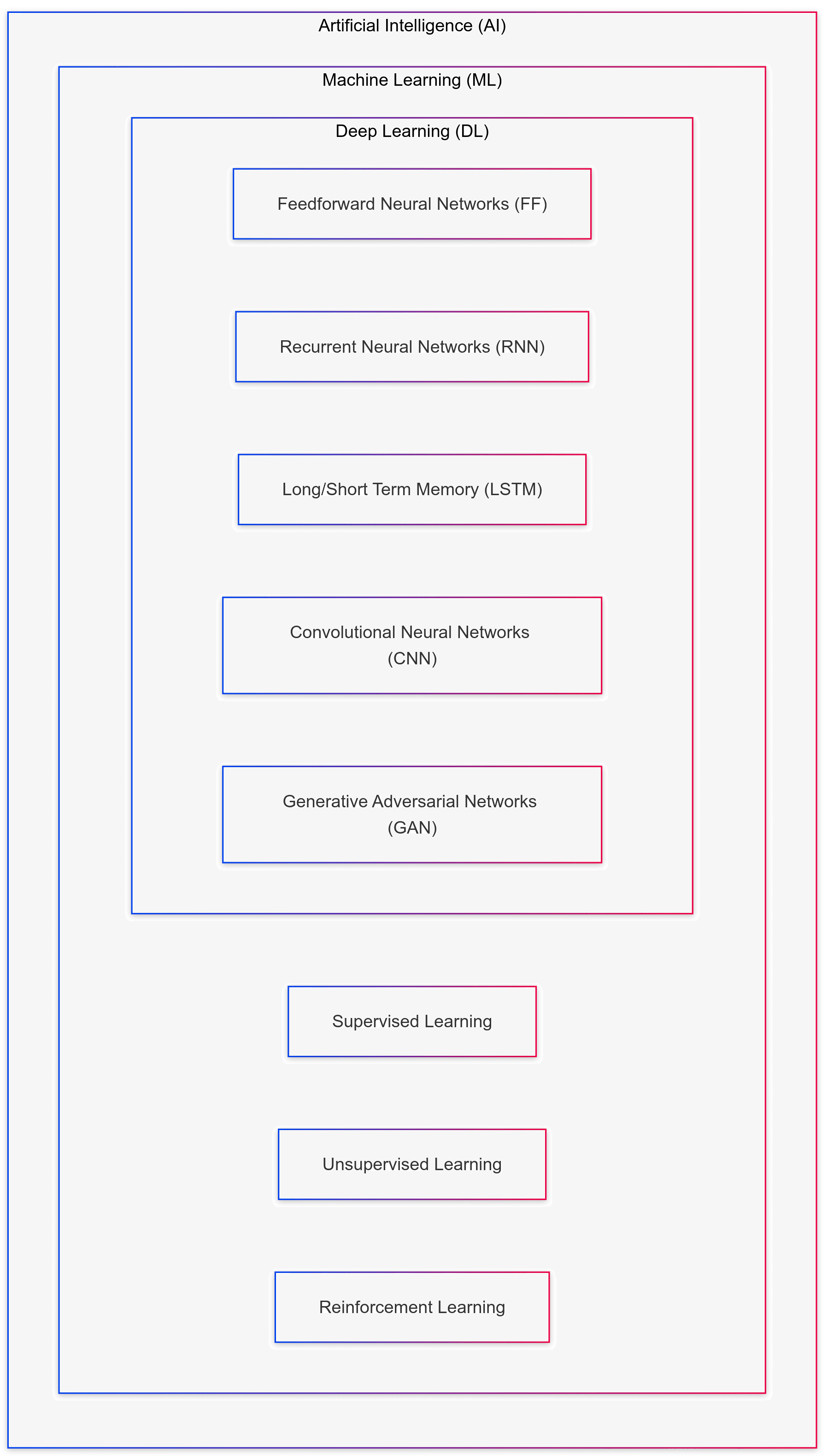
This diagram illustrates the hierarchy within Artificial Intelligence (AI), showcasing how Machine Learning (ML) and Deep Learning (DL) fit within AI. It highlights various deep learning models, such as Feedforward Neural Networks, Convolutional Neural Networks, and Generative Adversarial Networks, as well as learning types like Supervised, Unsupervised, and Reinforcement Learning. Each layer represents increasingly specialized areas, with AI at the top as the broadest field, narrowing down to specific algorithms and techniques within DL.

1. Machine Learning

Machine Learning (ML) is a subset of AI that focuses on developing algorithms that enable machines to learn from data and improve their performance over time without being programmed for each task. Within ML, there are different types of learning.

1.1 Supervised Learning

Supervised learning is a type of machine learning where we work with a dataset that includes the input data (features) and the correct answers (labels). The goal is to train a model to predict the labels when given new input data. Features are individual information or variables used as inputs to make predictions. Think of features as the characteristics or attributes of the data that you believe will help make a prediction.

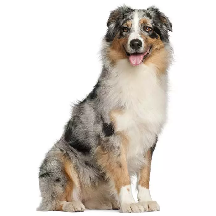
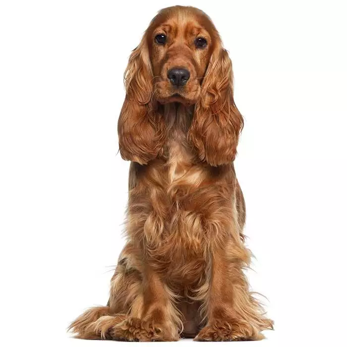
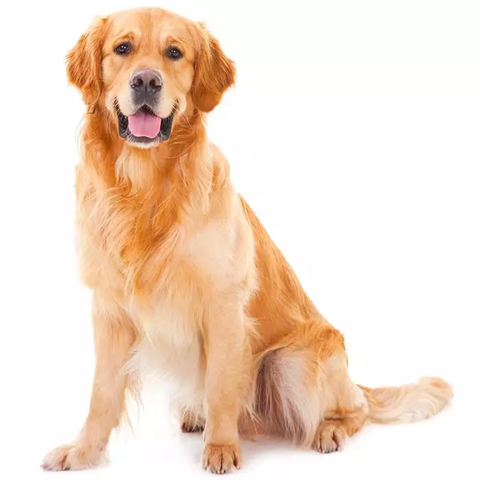
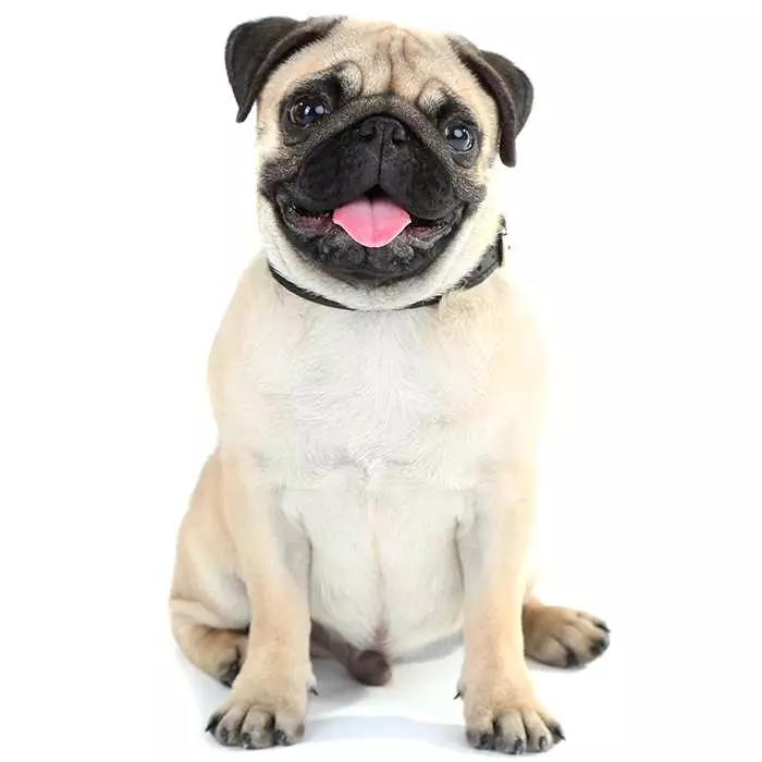
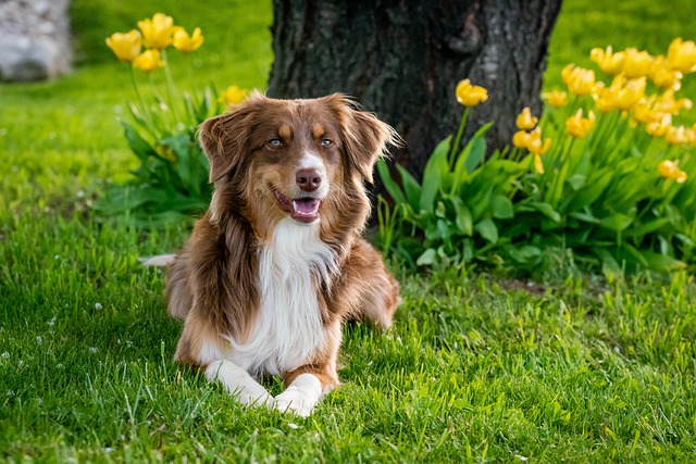
For example, in a dataset about dogs, the features might include the animal’s size, the shape of its ears, the length of its tail and coat, and the shape of its head. The label could be the dog’s breed, the specific outcome, or the value you want the model to predict based on the features.

To make this prediction process happen, you need a large dataset containing many examples of dogs with known features and labels. This data is then fed into a model, which uses algorithms to learn from the patterns in the data. The model uses this learning to predict new data where the label is unknown, such as identifying a dog’s breed based on its physical characteristics.

Feature: Size

Feature: Ear Shape

Feature: Tail Length

Feature: Coat Length

Feature: Head Shape

Model

Predict: Australian Shepherd

Predict: Cocker Spaniel

Predict: Golden Retriever

Predict: Pug

Example Training Data

Image	Size	Ear Shape	Tail Length	Coat Length	Head Shape	Breed (Label)
	Medium	Semi-Erect	Short	Medium	Square	Australian Shepherd
	Medium	Floppy	Medium	Long	Round	Cocker Spaniel
	Large	Floppy	Long	Long	Broad	Golden Retriever
	Small	Button	Curled	Short	Round	Pug

Now that the model has been trained let’s see how it predicts the breed of a new dog.

(Unknown Breed)

A user uploads an image of a dog. The model processes the image by extracting key features:

Image	Size	Ear Shape	Tail Length	Coat Length	Head Shape	Predicted Breed
🐕❓	Medium	Semi-Erect	Short	Medium	Square	Australian Shepherd (90%)

The model detected that the dog’s ear shape, tail length, coat length, and head shape closely matched the patterns it learned from Australian Shepherds. It calculated probabilities for different breeds and found that Australian Shepherd had the highest match (90%).

1.1.1 Regression

Regression is a type of supervised learning that aims to predict a continuous numerical value based on input features. For example, let’s say we want to predict the selling price of a house. In a hypothetical scenario, the house’s price depends on location, square footage, age, condition, and the number of bathrooms and bedrooms.

Example Dataset

Bedrooms	Square Footage	Location	Age of House (Years)	Bathrooms	Condition	Selling Price ($)
3	1500	1	10	2	3	600,000
4	2000	2	5	3	3	750,000
2	1000	1	20	1	3	450,000
5	3000	3	2	4	4	1,400,000

In this dataset:

Location is encoded as a numerical value ranging from 1 to 3: 1=Urban, 2=Suburban, 3 = Rural

Condition is also encoded numerically, where: 1 = Poor, 2 = Fair, 3 = Good, 4 = Excellent

Each house in the dataset is represented as a vector of features. For example:

• House 1: [3, 1500, 1, 10, 2, 3]
• House 2: [4, 2000, 2, 5, 3, 3]…

Using this dataset, you can train a regression model. The model learns to associate the house’s features (like the number of bedrooms, bathrooms, and square footage) with the target value (selling price).

The model might learn an equation like this:

\[ \text{Price} = w_1 \times \text{Bedrooms} + w_2 \times \text{Square Footage} + w_3 \times \text{Location} + w_4 \times \text{Age of House} + w_5 \times \text{Bathrooms} + w_6 \times \text{Condition} + b \]

\[ w_1, w_2, \dots, w_6 \text{ are the weights learned by the model, representing how much each feature impacts the price.} \]

\[ b \text{ is the bias term.} \]

Once the model is trained, you can use it to predict the price of a new house.

For example, consider a new house with the following features:

• Bedrooms: 3
• Square Footage: 1800
• Location: Suburban (encoded as 2)
• Age of House: 8 years
• Bathrooms: 2
• Condition: Good (encoded as 3)

These features can be represented as a vector: [3,1800,2,8,2,3][3, 1800, 2, 8, 2, 3][3,1800,2,8,2,3]

The model processes these inputs and predicts the house price, for example, $650,000.

Regression is often used to predict future stock prices, housing prices, GDP, and economic growth, forecast temperatures, and calculate insurance premiums.

1.1.2 Classification

Imagine you have a dataset about dogs, where the features include the dog’s size, the shape of its ears, the length of its tail and coat, and the shape of its head. If you want to predict the breed of the dog based on these features, this would be a classification problem. In this case, the label is the breed of the dog, which is a specific category. The model learns from the data and classifies a new dog into a breed based on physical characteristics. For example, given the features, the model might classify a dog as a Pug or a Golden Retriever. (see example above)

Classification tasks are widely used in various fields to, for example, identify diseases from medical images, recognize faces, or enable autonomous vehicles to detect and classify objects on the road.

If you want to try image labeling, use CVAT, Labelme, or LabelBox tools.

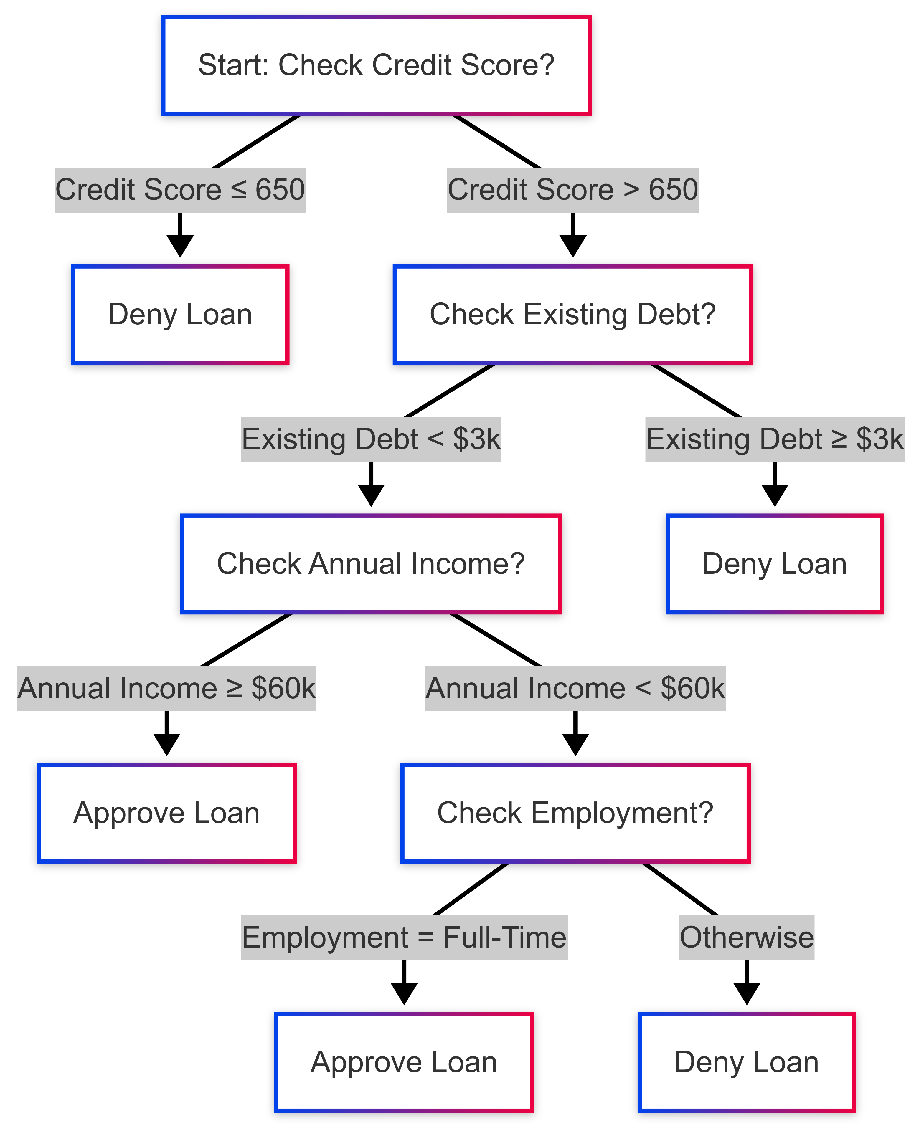
1.1.3 Decision Trees

Decision trees make splits in your data based on feature thresholds. Each split aims to maximize purity in the resulting subsets (using Gini impurity or entropy for classification). It’s like playing a game of “20 Questions,” where each question is a feature-based decision.

Example Scenario: Approving or Denying Loan Applications.

Suppose you have a dataset of loan applicants that includes features like credit score, annual income, employment status, and existing debt. The goal is to predict whether to approve (Yes) or deny (No) each application:

Credit Score	Annual Income	Employment Status	Existing Debt	Loan Approved?
750	$80,000	Full-Time	$2,000	Yes
620	$45,000	Part-Time	$5,000	No
680	$60,000	Full-Time	$1,000	Yes
550	$35,000	Unemployed	$6,000	No

A decision tree might learn rules such as, “If Credit Score > 650 and Existing Debt < $3,000, Approve Loan.” However, trees can overfit if they grow too large. Pruning techniques or setting limits on tree depth can help generalize better.

1.1.4 Random Forest

A Random Forest is like having a committee of decision trees working together to decide whether to approve or deny a loan. Instead of training just one tree on the entire loan dataset, the algorithm builds multiple trees, each trained on different data samples and other random subsets of features (like credit score, income, existing debt, and employment status). After all these trees have been trained, they each predict “Approve” or “Deny.” The forest then takes a vote: if most trees say “Approve,” the loan is approved; otherwise, it’s denied. This process lowers the risk of overfitting because any specifics in one tree’s subset of data are averaged out when you combine all the trees. It also typically produces more accurate predictions than just a single decision tree. For lenders, the result is a more consistent and reliable model that generalizes better to new, unseen applicants, improving overall loan-approval accuracy.

In this chart, each decision tree has its accuracy. The random forest combines these trees and can often achieve even higher accuracy.

1.1.5 Support Vector Machines (SVM)

SVMs aim to find a hyperplane that separates classes with the maximum margin. This is extremely powerful when the data is linearly separable. For data that isn’t linearly separable, you can apply the “kernel trick” to project it into a higher-dimensional space where a separating boundary might exist.

Example: Classifying emails as “Spam” or “Not Spam” based on text features (e.g., word counts, presence of suspicious links). An SVM can map these word frequencies into a higher-dimensional space and create a boundary separating spam from non-spam emails.

The decision boundary (hyperplane) in a 2D plot might be a line. In higher dimensions, it’s a hyperplane that separates the two classes.

1.1.6 k-Nearest Neighbors (k-NN)

k-NN is a lazy learning algorithm: it doesn’t create an explicit model. Instead, it stores the training instances and classifies a new data point by a majority vote of its “k” nearest neighbors in feature space.

Example: Recommending a movie to a new user by looking at the “k” of the most similar users (neighbors) who liked identical films.

In this simplistic illustration, if k = 3, the new user at (2,3) might be closer to the Comedy Fans cluster, so the algorithm recommends a comedy movie first.

1.4.5 Naive Bayes

Naive Bayes applies Bayes’ Theorem, simplifying calculations by assuming features are conditionally independent (which is rarely true in reality, but works surprisingly well in practice). Popular for text classification tasks like spam filtering or sentiment analysis.

Example: Sentiment analysis on product reviews: given the frequency of certain words, predict if a review is “Positive” or “Negative.”

The model might learn that words like “amazing,” “wonderful,” or “highly recommend” are positively correlated with a 5-star sentiment, while words like “poor,” “awful,” or “never again” are negatively correlated.

1.2 Unsupervised Learning

Unsupervised Learning is another subset of machine learning. Unsupervised learning involves algorithms that learn independently without labels or prior training. These models are provided with raw, unlabeled data and must independently identify patterns, similarities, and differences. One type of unsupervised learning is clustering, where the machine will try to cluster the data it receives and create groups.

Let’s say you are an e-commerce store that wants to understand your customers’ behavior better and improve your marketing strategies. However, you don’t have labeled data that categorizes your customers into predefined segments. This is where unsupervised learning, specifically clustering, can be helpful.

You start by collecting raw data on your customers, including information like:

• Purchase History: Total number of purchases, frequency, average purchase value. ( for example, from Woocommerce)
• Browsing Behavior: Pages visited, time spent on the website, products viewed. ( from Google Analytics)
• Demographics: Age, gender, location, income level. (from Google Analytics or surveys)

This data is unlabeled, meaning there’s no predefined category or segment for each customer.

1.2.1 K-Means Clustering Algorithm

You can apply a clustering algorithm, such as K-means clustering, to the dataset. The algorithm scans the data and tries to identify patterns, similarities, and differences among the customers. Based on these patterns, the algorithm groups customers into clusters. Each cluster represents a group of customers with similar characteristics.

After running the clustering algorithm, you might find that your customers are grouped into the following clusters:

Cluster 1: High-frequency buyers who spend much per transaction but visit the site less frequently. Customers in the first cluster should receive exclusive discounts or loyalty rewards.

Cluster 2: Regular visitors with a moderate purchase frequency and average spending per transaction. Customers in this cluster may purchase more if they receive more personalized recommendations.

Cluster 3: Occasional visitors who browse a lot but purchase infrequently and have a lower average spend. Target customers with ads or promotional emails, such as a cart reminder email campaign.

This is just an example; the clusters will depend on the e-commerce platform’s data, and the marketing strategies will depend on the budget and the store’s specific situation.

1.2.2.Density-Based Spatial Clustering of Applications with Noise (DBSCAN)

One limitation of K-Means clustering is that it assumes clusters are spherical and of similar sizes, which isn’t always the case in real-world data. Density-Based Spatial Clustering of Applications with Noise (DBSCAN) is an alternative clustering algorithm that identifies clusters based on density rather than predefined shapes.

Imagine you run a retail store with both online and physical locations. You want to optimize your regional marketing efforts by understanding where your customers are concentrated. However, your customer location data is complex, with some densely populated areas and others more sparse.

You start by collecting raw customer location data, including:

• Shipping addresses from past purchases.
• In-store visit logs, if available.
• Mobile app location check-ins from loyalty program users.

This dataset is unlabeled, meaning you don’t know which geographical clusters exist.

You apply DBSCAN to your dataset. Unlike K-Means, DBSCAN doesn’t require you to predefine the number of clusters. Instead, it groups customers based on densely populated regions while ignoring outliers.

After running DBSCAN, you may find clusters such as:

• Cluster 1: Customers concentrated in large urban areas who prefer in-store pickup.
• Cluster 2: Suburban shoppers who purchase online and visit the store occasionally.
• Cluster 3: Remote or rural customers who rely heavily on home delivery.

By analyzing these clusters, you can adjust your marketing efforts—offering in-store discounts for urban customers, targeted promotions for suburban buyers, and free shipping for rural customers.

To learn more about clustering, follow this Google Cloud Course.

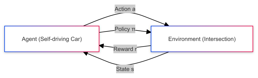
1.3 Reinforcement Learning

Reinforcement learning involves an agent interacting with an environment over time. At each step, the agent observes the environment, takes action, and receives feedback as a reward. The process then repeats: the agent makes another observation, takes another action, and gets another reward. The agent’s behavior is guided by a policy, a rule, or a function that decides what action to take based on the current observation. The main goal of reinforcement learning is to develop effective policies that produce the best possible rewards.

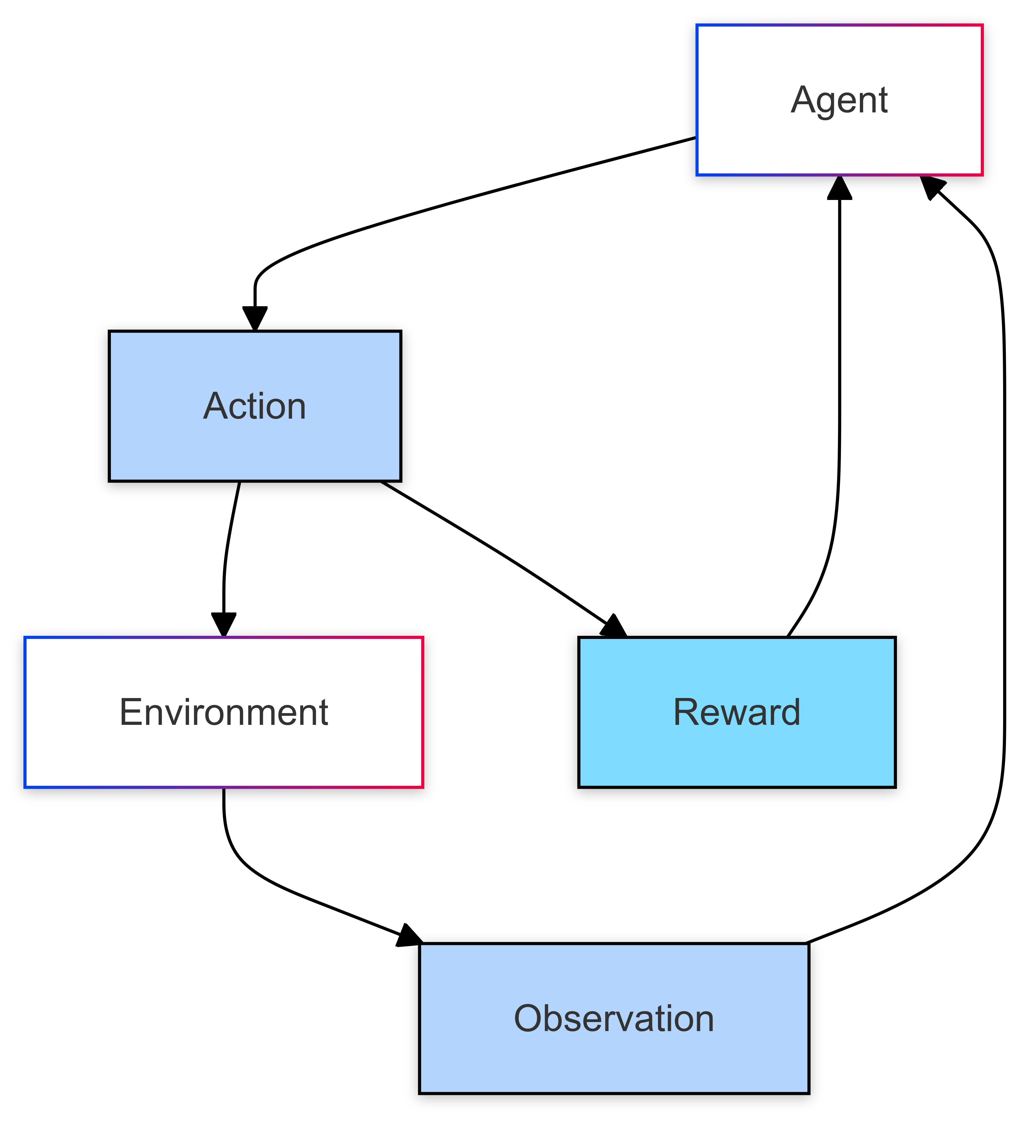
For example, reinforcement learning works in a self-driving car by having the car, or agent, interact with its environment—the road, other vehicles, pedestrians, and traffic signals. The car constantly receives observations from its sensors, like cameras and radar, which provide information about its surroundings. Based on these observations, the car decides what action to take, such as turning, braking, or accelerating.

After each action, the car receives feedback (reward) indicating how well it performed. For example, safely stopping at a red light might earn a positive reward, while getting too close to another vehicle could result in a negative reward. The car uses this feedback to learn over time, adjusting its strategy or policy to make better decisions in the future. The vehicle aims to maximize positive rewards, leading to safe and efficient driving.

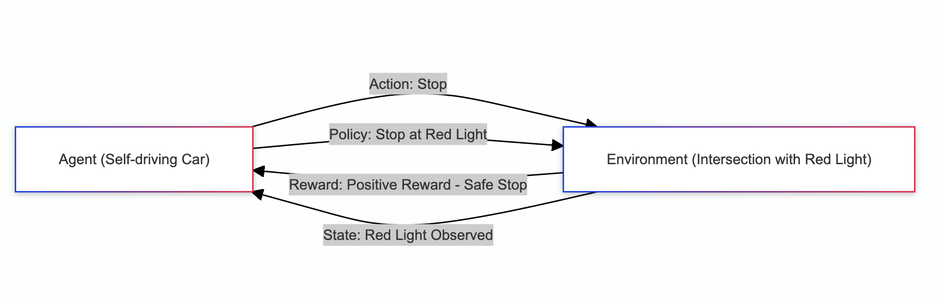
Example: A self-driving vehicle stopping at a red light.

The self-driving car is the agent that needs to make decisions. The environment is the intersection where the traffic light has turned red, signaling the car to stop. The vehicle decides to stop as it approaches the intersection because the light is red. This is the action it takes. The car observes the environment’s state, including the red light, the car’s position relative to the intersection, and possibly other cars stopping. The vehicle receives a positive reward for stopping because it follows the traffic rules and avoids a potential accident. The car’s policy guides it to stop whenever it encounters a red light at an intersection. Over time, it learns to stop correctly and consistently at red lights.

Because driving involves many unpredictable, complex scenarios, cars cannot completely self-drive without making mistakes. According to the Society of Automobile Engineers, the highest level of autonomous vehicles for sale in the USA is level 3 cars, which can self-drive. Still, humans must be prepared to take over when necessary. Only the Honda Legend, the Mercedes EQS, and the S-class are approved for level 3 autonomous driving in the USA.

To learn more about Mercedes’ self-driving technologies, watch this video: